Previously we talked about how to improve the contrast of a grey scale image. Subsequently we looked at how we could apply similar techniques on color images [INSERT LINK]. During these two articles, we used OpenCV’s equalizeHist function to equalize a pixels’ intensity across the entire image. In other words, we equalized across the entire spectrum of pixel intensity globally. Unfortunately using this approach has its’ drawback. As we saw before, certain areas becoming over exposed, or in some cases wrong colors appearing. Conversely, instead of equalizing globally, what if we could limit to a smaller area of the picture? Better still, what if we could add a threshold to limit the amount of change made to each pixel. Therefore today, we’d like to talk about Color Image Histograms – CLAHE (Contrast Limited Adaptive Histogram Equalization)
Setup pre-requisites and load background libraries
To begin with, we import OpenCV and Numpy libraries. Furthermore, we create our helper function to display images using Matplotlib in Jupyter Lab.
import cv2
import numpy as np

#The line below is necessary to show Matplotlib's plots inside a Jupyter Notebook
%matplotlib inline

from matplotlib import pyplot as plt

#Use this helper function if you are working in Jupyter Lab
#If not, then directly use cv2.imshow(<window name>, <image>)

def showimage(myimage, figsize=[10,10]):
    if (myimage.ndim>2):  #This only applies to RGB or RGBA images (e.g. not to Black and White images)
        myimage = myimage[:,:,::-1] #OpenCV follows BGR order, while matplotlib likely follows RGB order

    fig, ax = plt.subplots(figsize=figsize)
    ax.imshow(myimage, cmap = 'gray', interpolation = 'bicubic')
    plt.xticks([]), plt.yticks([])  # to hide tick values on X and Y axis
    plt.show()
As the last preparatory step, we read in our image
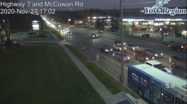
colorimage = cv2.imread("Hwy7McCowan Night.jpg")
showimage(colorimage)
How to – Color Image Histogram CLAHE
At this point instead of applying EqualizeHist over the entire image, we will instead create a CLAHE object. This built-in model of OpenCV is similar and allows us to pass in two additional key parameters. Firstly, we need to specify our input image. Secondly, we can define a ClipLimit (threshold for contrast change). Lastly, we provide the local area size to which equalization will be performed.
# We first create a CLAHE model based on OpenCV
# clipLimit defines threshold to limit the contrast in case of noise in our image
# tileGridSize defines the area size in which local equalization will be performed
clahe_model = cv2.createCLAHE(clipLimit=3.0, tileGridSize=(8,8))
Once again, we apply our CLAHE model against each channel of our color image
# For ease of understanding, we explicitly equalize each channel individually
colorimage_b = clahe_model.apply(colorimage[:,:,0])
colorimage_g = clahe_model.apply(colorimage[:,:,1])
colorimage_r = clahe_model.apply(colorimage[:,:,2])
Afterwards, don’t forget to stack our three arrays back into a single BGR image
# Next we stack our equalized channels back into a single image
colorimage_clahe = np.stack((colorimage_b,colorimage_g,colorimage_r), axis=2)
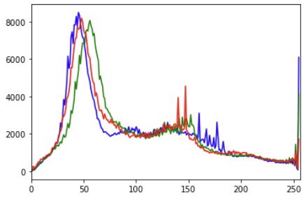
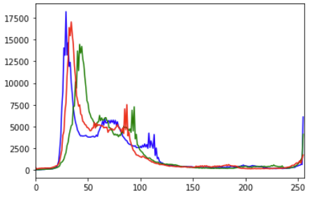
At this point we can plot our color image histogram to see what has happened. The code is similar for plotting the histogram of our original image. See our earlier post on
# Using Numpy to calculate the histogram
color = ('b','g','r')
for i,col in enumerate(color):
    histr, _ = np.histogram(colorimage_clahe[:,:,i],256,[0,256])
    plt.plot(histr,color = col)
    plt.xlim([0,256])
plt.show()

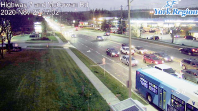
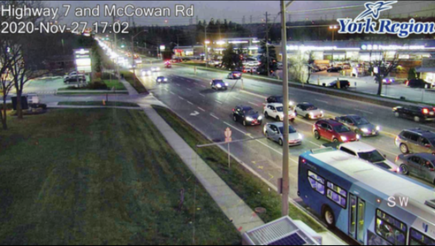
CLAHE processed image 
Original Image before CLAHE
Finally, the moment we have been waiting for. Comparatively, have we improved our image contrast without losing detail?
# Show all three images as comparison
showimage(colorimage)
showimage(colorimage_e)
showimage(colorimage_clahe)

Summary
Comparatively amongst the two different contrast improving methods on color image histograms, the result of CLAHE are better. Not only did we reduce the over exposure in the upper right, most of the details were retained. Additionally the contrast of cars behind the bus was improved without being drowned out by the car’s high beam. Furthermore look closely at the lawn on the lower left of the image. Some of the details on the lawn can be clearly seen, whilst dis-coloration did not occur.
In conclusion, the result of Contrast Limited Adaptive Histogram Equalization (CLAHE) produces better results.

