Support Vector Machines

Support Vector Machines is yet another model that is commonly used to solve data classification problems. Previously, we looked at different approaches to classification such as K-means clustering, or Decision Trees, as well as how to use Random Forests. Unquestionably we recommend checking out these posts as well.

Analogous to all other classification models, Support Vector Machines is based on the general concept: Can we identify an optimal hyperplane that will enable us to separate one group of data points from each other? In other words, given a n-feature dataset we can represent this data in n-dimension space. On this occasion we would like to find a hyperplane or surface that can separate these datapoints.

Support Vector Machine – Concept

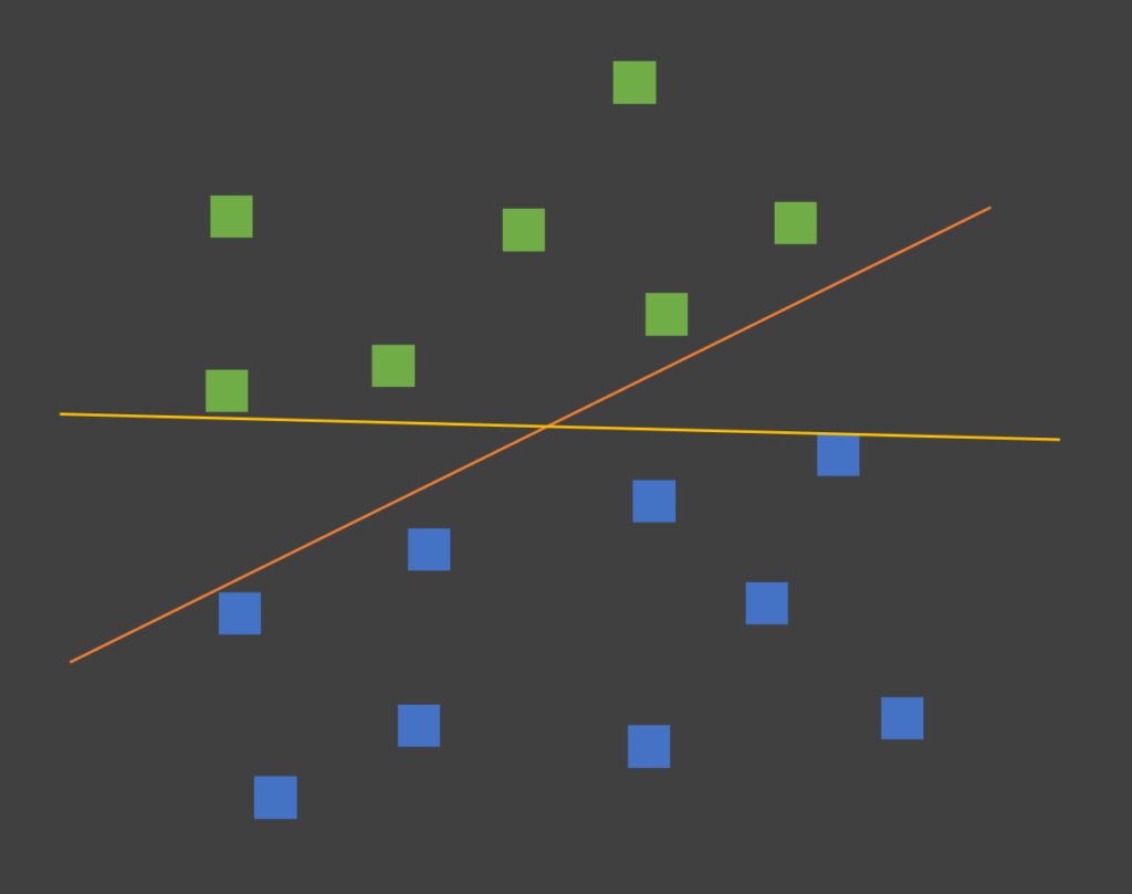
As an illustration of the concept, imagine a dataset with only 2 features in our dataset. Additionally, each datapoint belongs to one of two classes. In this case, we could represent the dataset in a 2D scatter plot like below. The color of the datapoint tells us which class it belongs to. As can be seen we only have two classes in our example. Straightaway you may realize we could draw a line that would bisect our data to allow us to easily separate each class. At the same time, we could actually draw infinite number of lines to separate our data. For example we have a yellow and an orange line in our diagram.

Support Vector Machines Concept 1 - Data points in 2D Space belonging to two classes

Support Vectors and Hyperplane

The key concept of the SVM is in finding the “Optimal” line that separates our data. Moreover “Optimal” is defined as the hyperplane (or line 2D space) that maximizes the margin between the lines and the datapoints. Furthermore, Support Vectors are those datapoints that are closest to our hyperplane.

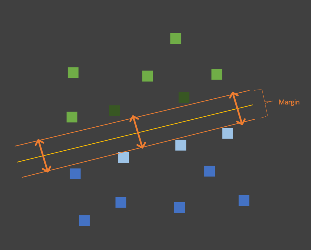
Support Vector Machines Concept 2 - Hyperplane and Margin

Hence in reality, only a small number of datapoint actually influence how we separate our data into classes. Likewise as long as they do not cross the margins, all other datapoints can move and it would have no influence on our hyperplane.

Support Vector Machines Concept 3 - Support Vectors

Support Vector Machine in practice

All things considered we now demonstrate how easy it is to start using Support Vector Machines by leveraging the libraries available in Scikit-learn. First thing to remember is to import the necessary libraries for our example.

from sklearn import svm
import matplotlib.pyplot as plt
from sklearn.datasets import make_blobs
import numpy as np

Subsequently we want to prepare our dataset. For the purpose of our discussion, we will first create a dataset of 50 datapoints across two classes.

# The make_blobs function allows us to quickly generate datasets based on the number of centers/classes
num_class=2
Data1, Label1 = make_blobs(n_samples=50, centers=num_class, random_state=3)

Now that we have our dataset, we need to create and train our model. Explicitly in our discussion we want to work with a linear kernel. Of course other kernels are also available and we will look into those later.

MySVC1 = svm.SVC(kernel="linear",C=1)
MySVC1.fit(Data1,Label1)

Visualizing our SVM

Generally, at this point we would run the predict function of our trained model to test its’ accuracy (e.g. MySVC1.predict(testdata)). This time instead we will create a helper function. It will take the prediction results and plot it’s output. In reality this will allow us to better visualize the output from our SVM.

def chart_svm(model, Data, Label, num_class=2):
    fig, ax = plt.subplots()
    ax.scatter(Data[:,0],Data[:,1], s=40,c=Label,cmap=plt.cm.Paired)

    # Based on our axis, to plot the hyperplane(s) of our dataset
    ax = plt.gca()
    xlim = ax.get_xlim()
    ylim = ax.get_ylim()
    xx, yy = np.meshgrid(np.linspace(xlim[0], xlim[1], 50),
                         np.linspace(ylim[0], ylim[1], 50))

    # Perform model prediction and store it as "Z"
    Z = model.predict(np.c_[xx.ravel(), yy.ravel()])
    Z = Z.reshape(xx.shape)
    plt.contourf(xx, yy, Z, alpha=0.3, cmap=plt.cm.coolwarm)

    # Define Z to plot hyperplane if num_class==2
    if num_class==2:
        Z = model.decision_function((np.c_[xx.ravel(), yy.ravel()]))
        Z = Z.reshape(xx.shape)                           
        plt.contour(xx, yy, Z, colors='k', levels=[-1, 0, 1], alpha=0.5,
                    linestyles=['--', '-', '--'])
    plt.show()

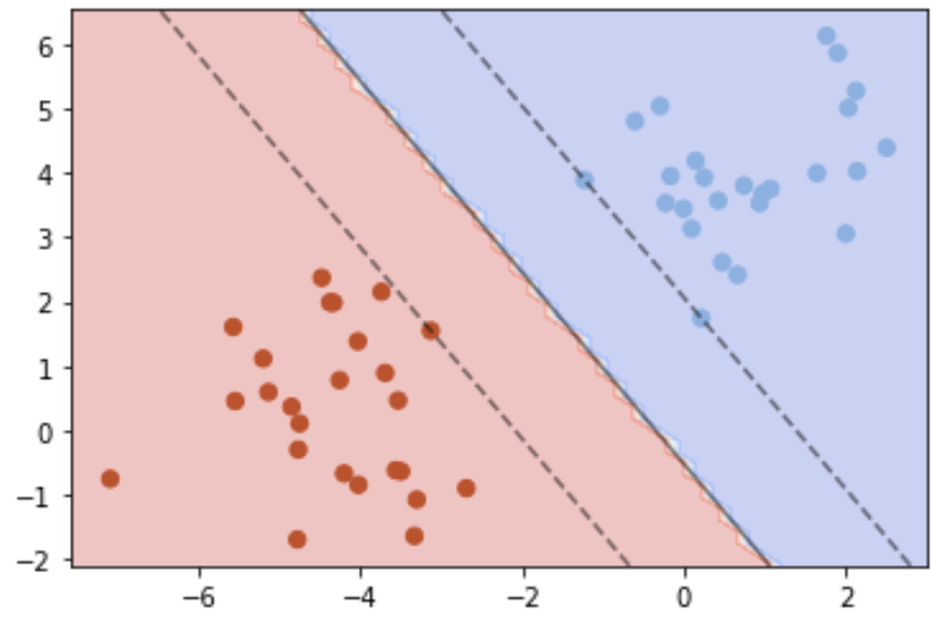
Important to realize within our function above, we perform our prediction. Furthermore this is saved as a variable “Z” and used to make our plot. Finally we call our function to plot the results.

chart_svm(MySVC1, Data1, Label1)

Multi-class Linear SVM

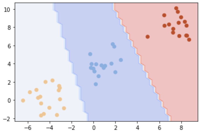
Now that we’ve seen how SVMs work with a simple 2 class linear kernel, we can also quickly demonstrate how multi-class SVMs work.

# Additionally we create a dataset but this time with 3 centers/classes
Data2, Label2 = make_blobs(n_samples=50, centers=3, random_state=3)
MySVC2 = svm.SVC(kernel="linear",C=100)
MySVC2.fit(Data2,Label2)
chart_svm(MySVC2, Data2, Label2, num_class=3)