Color Space
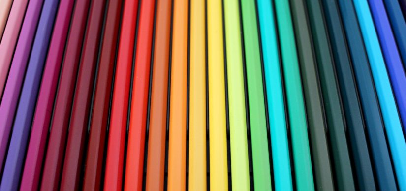
Color is a human perception and describes the visible spectrum of light that is reflected off the surface of any object. With the advancement of computers, we went from monochrome to color displays. This led the industry to come up with different ways to tell the computer what is “color”. Consequently the many “Color Space” has emerged. When working with images there are 3-4 most commonly used color spaces. In our earlier post on “How to load and save images”, we already saw some of them. For instance, greyscale (black and white) images has “color” represented as a numerical value normally between 0 to 255 (8bit). Another color space we’ve encountered in the past is RGB (Red Green Blue), or in OpenCV BGR (Blue Green Red). Finally today we would like to introduce a fourth commonly used color space; namely HSV (Hue Saturation Value).
Color space – Hue Saturation Value (HSV)
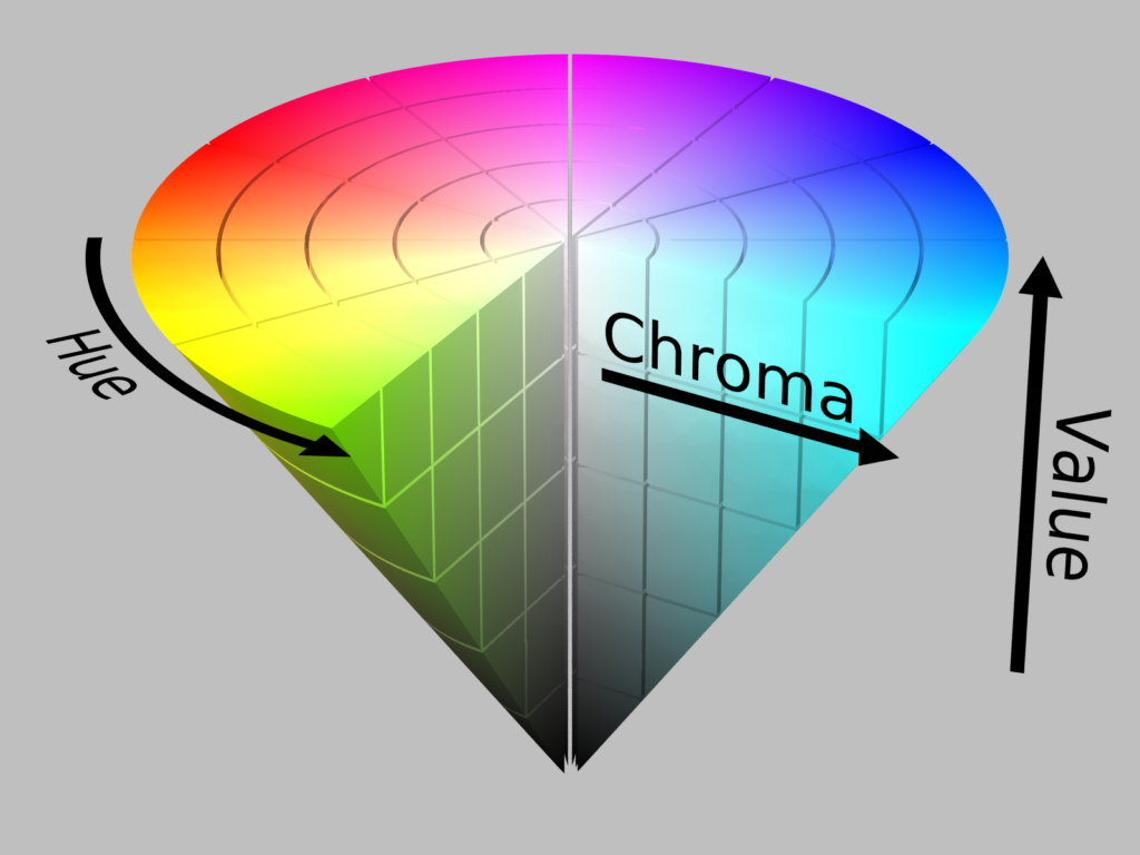
HSV as the name implies stores the value of color as a 3-tuple. H stands for Hue and is a single value to represent color from 0 to 360. Owing to this, Hue can be described as a circle based on its degree. S stands for Saturation (or sometimes called Chroma) and can also be described as how “gray” the color is. Finally V stands for Value or sometimes referred to as Brightness. Brightness as the name implies describes how white (bright) or black (dark) the color is. To illustrate and better visualize HSV, we visualize it as cone.
Advantages of using HSV
In view of several color spaces available to chose from, why would we introduce another one? In order to answer this question, we need to look back at RGB. Important to note is RGB uses all three channels in combination to represent color. As a result, dependent on the lighting conditions, the RGB values can fluctuate dramatically. In comparison, as HSV isolates color (Hue) from brightness, the Hue is less subject to fluctuations due to lighting conditions. To demonstrate this we show two pictures taken at different times of day.
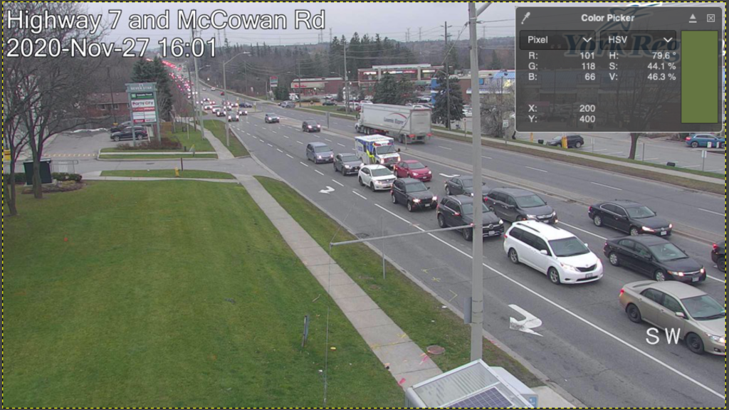
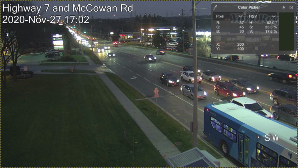
At this point we focus on the large patch of grass on the lower left of the image with the color picker displaying both RGB and HSV values on the same pixel. Notice how all RGB values displayed a large fluctuation of 30-65 (out of 256). In contrast, the Hue value of HSV only fluctuated by roughy 15 degrees (out 360). In other words, using RGB values the color fluctuated by about 17% while the Hue value only fluctuated by 4%.
Converting images between Color Space
Now that we understand why it may be advantageous to use HSV, the obvious question is how to convert images between color spaces. First we import the necessary libraries and optional function for displaying images in Jupyter notebooks and our image.
import cv2
import numpy as np

#Load our image
image = cv2.imread("Hwy7McCowan Day Colorpicker.png")

#The lines below is only necessary to show Matplotlib's plots inside a Jupyter Notebook
%matplotlib inline

from matplotlib import pyplot as plt

#Use this helper function if you are working in Jupyter Lab
#If not, then directly use cv2.imshow(<window name>, <image>)

def showimage(myimage):
    if (myimage.ndim>2):  #This only applies to RGB or RGBA images (e.g. not to Black and White images)
        myimage = myimage[:,:,::-1] #OpenCV follows BGR order, while matplotlib likely follows RGB order

    fig, ax = plt.subplots(figsize=[10,10])
    ax.imshow(myimage, cmap = 'gray', interpolation = 'bicubic')
    plt.xticks([]), plt.yticks([])  # to hide tick values on X and Y axis
    plt.show()
As an initial demonstration, we convert between BGR (the default representation in OpenCV) to grayscale
#Convert BGR to Grayscale
imagegray = cv2.cvtColor(image,cv2.COLOR_BGR2GRAY)
showimage(imagegray)
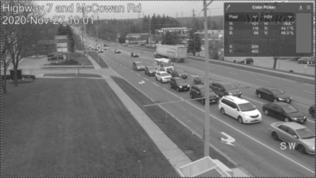
Next, we convert our image from BGR to HSV.
# Convert image to HSV
imageHSV = cv2.cvtColor(image,cv2.COLOR_BGR2HSV)
showimage(imageHSV)
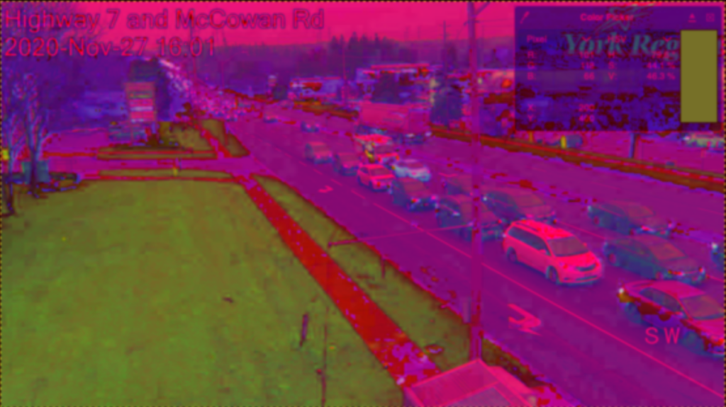
As shown above, using only a single line of code will allow us to convert the image between different color spaces. There are many additional options provided by OpenCV in cvtColor for color conversion at your disposal. As a last topic, we explore how HSV stored in python. To demonstrate this, we take the RGB values shown in our day time picture.
# We first take the same RGB values as shown from our Color Picker and record them in BGR
grass = np.uint8([[[66,118,101]]])

# Next we convert the values to HSV as before
hsv_grass = cv2.cvtColor(grass,cv2.COLOR_BGR2HSV)

# Finally print out converted values
print(hsv_grass)
[[[ 40 112 118]]]Evident from our original image, we expect the answer to come to (79.6, 44.1%, and 46.3%). Most important to note, HSV is stored as follows:
- H = [0:179] – In order to fit 360 degrees into 8 bit integer, the values are divided by 2 (e.g. 360/2)
- S = [0:255]
- V = [0:255]
In conclusion, with some simple math, we can see that H=40 is equivalent to 80 degrees. Likewise S=112/256 = 44% and V=118/256 = 46%. Obviously, by using 8 bit integers we can experience information lost due to rounding. A conversion into fp32 would help alleviate the issue if color accuracy is of utmost importance.

