Image Thresholding
As the name implies, image thresholding allows us to apply a certain “threshold” to determine whether each pixel is of interest to us or not. Consequently, there are many practical and useful applications of image thresholding. For example we can use this to create a mask in order to isolate certain parts of an image. Alternatively, it can also be a good means to reduce noise within an image. With this in mind, let’s see how to use this in OpenCV.
In general we always start with loading the necessary libraries as well as our helper function to display images when using Jupyter notebooks.
import cv2
import numpy as np

#The line below is necessary to show Matplotlib's plots inside a Jupyter Notebook
%matplotlib inline

from matplotlib import pyplot as plt

#Use this helper function if you are working in Jupyter Lab
#If not, then directly use cv2.imshow(<window name>, <image>)

def showimage(myimage):
    if (myimage.ndim>2):  #This only applies to RGB or RGBA images (e.g. not to Black and White images)
        myimage = myimage[:,:,::-1] #OpenCV follows BGR order, while matplotlib likely follows RGB order

    fig, ax = plt.subplots(figsize=[10,10])
    ax.imshow(myimage, cmap = 'gray', interpolation = 'bicubic')
    plt.xticks([]), plt.yticks([])  # to hide tick values on X and Y axis
    plt.show()
To begin with, let’s load our grayscale image

Suppose we wanted to focus on the form and remove the wood grain distraction from the background. Recall that grayscale images are only 2D arrays with values between 0 to 255. In other words, we could set a threshold where we assign a value (e.g. 255 or white) to all pixels above a certain value (e.g. 140).
# Example of applying Image Thresholding on a grayscale picture.
threshold = 140
assignvalue = 255 # Value to assign the pixel if the threshold is met
threshold_method = cv2.THRESH_BINARY

_, result = cv2.threshold(imagegray,threshold,assignvalue,threshold_method)

# Display the results
showimage(result)
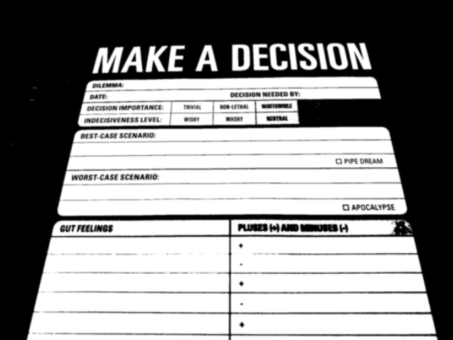
In the above example, we gave applied a “Global Threshold” universally across the entire image to test whether each pixel is above 140. In doing so, we started to get some good results. Notice how we got rid of the wood table in the background. There are many other Threshold Types available from OpenCV and you are all encouraged to check them out. Other available options include:
- cv2.THRESH_BINARY
- cv2.THRESH_BINARY_INV
- cv2.THRESH_TRUNC
- cv2.THRESH_TOZERO
- cv2.THRESH_TOZERO_INV
As the name implies another Threshold Type is the exact inverse of what we achieved “cv2.THRESH_BINARY_INV”, the results would be as the following:
threshold_method = cv2.THRESH_BINARY_INV
_, result = cv2.threshold(imagegray,threshold,assignvalue,threshold_method)

# Display the results
showimage(result)

Image Thresholding – How to decide on the threshold?
We produced a black and white image after applying a global threshold. Point often overlooked is how can we determine the threshold value? On the contrary, would it be possible not to provide a threshold and automatically identify the best threshold value? In other words, achieve freedom from choice? With this intention, OpenCV employs Otsu’s Binarization approach to image thresholding. Imagine a histogram that tallys the number of pixels with a certain value within your image. Subsequently, this histogram will contain peaks as certain pixels/colors may appear more frequently. Otsu’s binarization is an algorithm that automatically determines the best value to separate these peaks.
# Application of Otsu's Binarization method to automatically determine a threshold
_, result2 = cv2.threshold(imagegray,0,255,cv2.THRESH_BINARY+cv2.THRESH_OTSU)
showimage(result2)

By comparison with only using cv2.THRESH_BINARY, notice how our original guess of threshold=127 was quite good. Subsequently, by apply Otsu’s binarization method, we have improved. In this case, the lower right box labelled “Pluses and Minuses” was cleaner. Nevertheless, one caveat to highlight is the top of the form. Notice our original image contained five selection of varying brightness. With thresholding, it is very easy to omit needed elements if you are not careful. Based on this, we need a more sophisticated approach.
Masking and Image Thresholding for color images
At this point, we have seen how to use Image Thresholding on a grayscale image. This can be useful to help us further highlight or isolate parts of an image that is of interest. However, this begs the question how can we perform image thresholding on colored images. Consequently we introduce the concept of masking and how we can use this to isolate colored pixels of interest. In order to demonstrate this, we take an image of a young lady in the forest.
reddress = cv2.imread("RedDress1.jpg")
showimage(reddress)
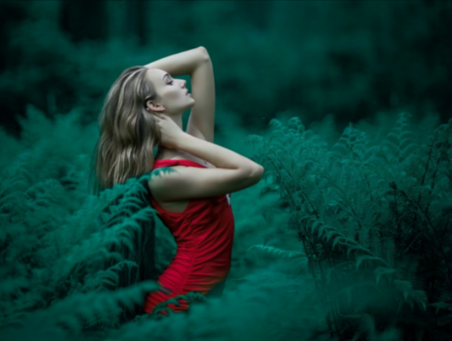
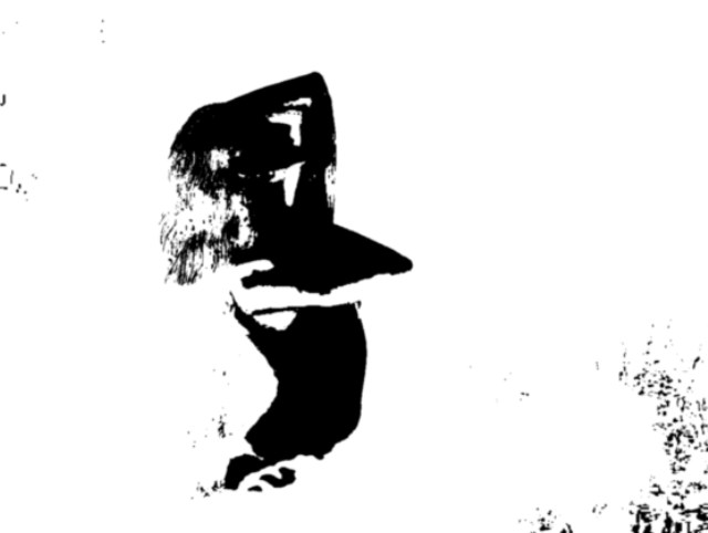
Seeing that the image is predominantly green with a lady in a red dress. In order to isolate her from the rest of the image, we could build a mask that consisted of all the green pixels. Alternatively we could have went with all red pixels and the different skin tones. Since it is easier with the former approach, we proceed in this manner. A mask is a matrix that shows pixels of interest in white (255), and those that are not interesting in black (0).
As there are many shadows and highlight in our image. Consequently we want to work in HSV space to better isolate the forest.
# Convert BGR to HSV
reddress_hsv = cv2.cvtColor(reddress, cv2.COLOR_BGR2HSV)

# Remember that in HSV space, Hue is color from 0..180. Red 320-360, and 0 - 30.
# We keep Saturation and Value within a wide range but note not to go too low or we start getting black/gray
lower_green = np.array([30,40,0])
upper_green = np.array([100,255,255])

# Using inRange method, to create a mask
mask = cv2.inRange(reddress_hsv, lower_green, upper_green)
showimage(mask)
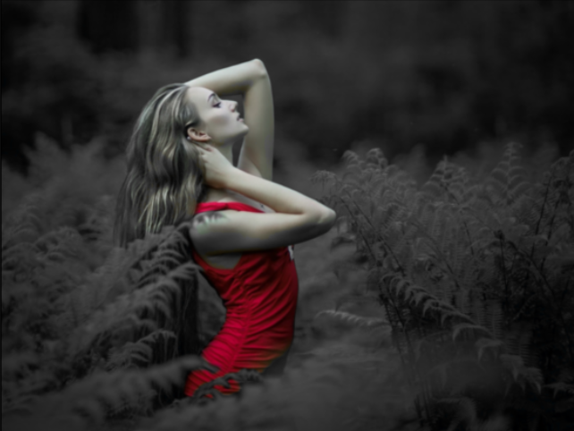
Black and White photo with color
Once we have a mask of the forest, we can proceed to process our image. Moreover our goal is to make a black and white photo with only the lady in color. By and large, this enables us to give more focus and pop to the lady in our image. At first, we will take our original image and convert them into a 3 channel grayscale image.
# We first convert our image into a 3 channel Grayscale image
reddress_gray = cv2.cvtColor(reddress,cv2.COLOR_BGR2GRAY)
reddress_gray = cv2.cvtColor(reddress_gray,cv2.COLOR_GRAY2BGR)

# notice we should have 3 channels even for our grayscale image
print(reddress_gray.shape)
(963, 1275, 3)Next, we will apply our mask to extract a grayscale version of the forest.
# We extract the gray scale version of our forest background
forest = cv2.bitwise_and(reddress_gray, reddress_gray, mask=mask)
showimage(forest)
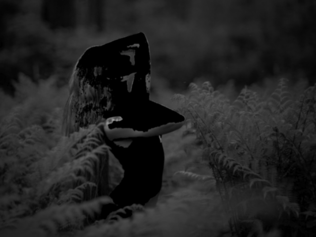
Afterwards, we will invert our mask to isolate the lady in our image.
# Next we invert our mask to isolate the lady in the red dress
mask_inv = mask
mask_inv[mask_inv==255] = 10
mask_inv[mask_inv==0] = 255
mask_inv[mask_inv==10] = 0

showimage(mask_inv)
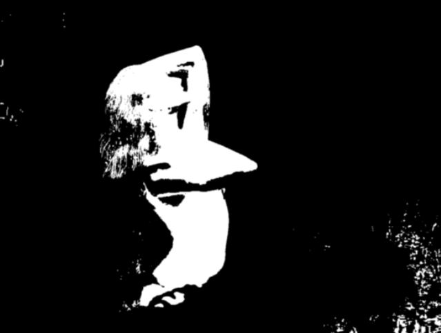
Similarly we apply our mask on our colored image to extract the image of our lady.
lady = cv2.bitwise_and(reddress,reddress, mask= mask_inv)
showimage(lady)

Finally all we need to do now is combine the image of the lady with the grayscale forest. Since black is 0 in our array, we simple perform matrix addition to create our desired image.
# As Black is 0, we can simply use matrix addition to add our two images back together
showimage(lady+forest)
