Basic Background Remover with OpenCV

In today’s blog we bring you through our recent journey in developing a basic background remover with OpenCV. Chiefly as we amass images for processing, we recognized there is a lot of undesirable background pixels in our images. Furthermore, it makes identifying the subject difficult at times. Therefore, we want to use our OpenCV skills to create a basic background remover. First and foremost, many of the concepts in this blog are based our previous posts. If you have not already, then please check our series on OpenCV. Accordingly, we created several background remover with OpenCV in order to find the solution that meets our needs.

Setting up pre-requisites

Since we will be using OpenCV, as before, we start by importing needed libraries and define our helper function

import cv2
import numpy as np

#The line below is necessary to show Matplotlib's plots inside a Jupyter Notebook
%matplotlib inline

from matplotlib import pyplot as plt

#Use this helper function if you are working in Jupyter Lab
#If not, then directly use cv2.imshow(<window name>, <image>)

def showimage(myimage):
    if (myimage.ndim>2):  #This only applies to RGB or RGBA images (e.g. not to Black and White images)
        myimage = myimage[:,:,::-1] #OpenCV follows BGR order, while matplotlib likely follows RGB order
        
    fig, ax = plt.subplots(figsize=[10,10])
    ax.imshow(myimage, cmap = 'gray', interpolation = 'bicubic')
    plt.xticks([]), plt.yticks([])  # to hide tick values on X and Y axis
    plt.show()

Background Remover with OpenCV – Method 1

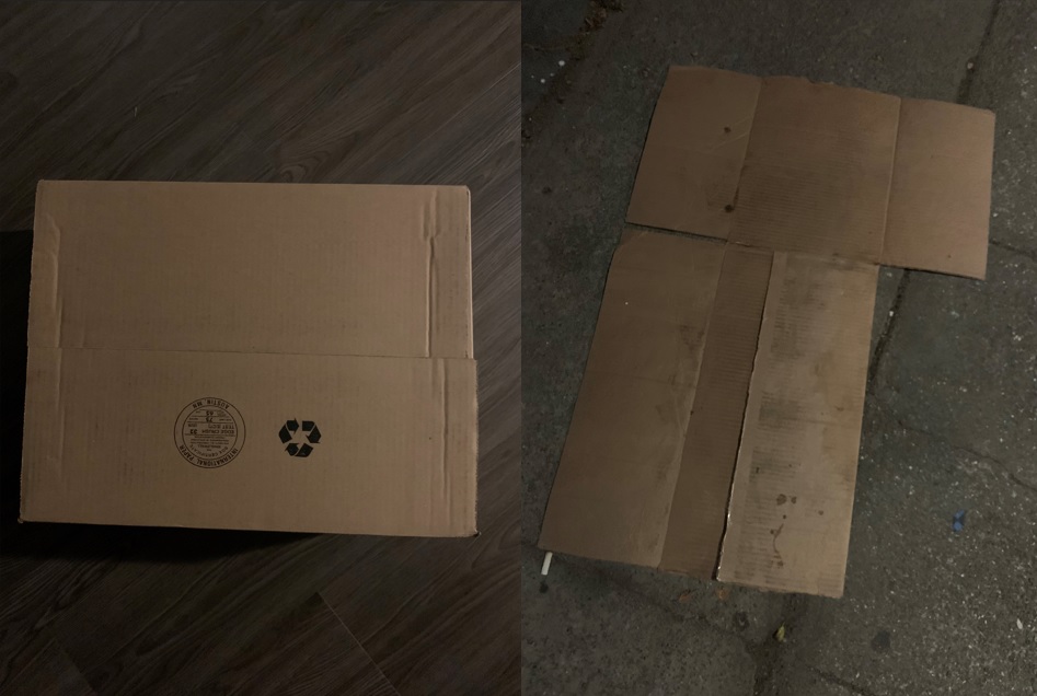
To begin with, our first background remover focuses on how to clean up images with background noise. Specifically poor lighting conditions or a busy backdrop can lead to very noisy backgrounds.

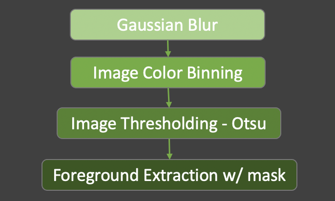
Based on this, we designed our background remover with the following strategy:

1. Perform Gaussian Blur to remove noise
2. Simplify our image by binning the pixels into six equally spaced bins in RGB space. In other words convert into a 5 x 5 x 5 = 125 colors
3. Convert our image into greyscale and apply Otsu thresholding to obtain a mask of the foreground
4. Apply the mask onto our binned image keeping only the foreground (essentially removing the background)

Given these points, our background remover code ended up as follows:

def bgremove1(myimage):

    # Blur to image to reduce noise
    myimage = cv2.GaussianBlur(myimage,(5,5), 0)

    # We bin the pixels. Result will be a value 1..5
    bins=np.array([0,51,102,153,204,255])
    myimage[:,:,:] = np.digitize(myimage[:,:,:],bins,right=True)*51

    # Create single channel greyscale for thresholding
    myimage_grey = cv2.cvtColor(myimage, cv2.COLOR_BGR2GRAY)

    # Perform Otsu thresholding and extract the background.
    # We use Binary Threshold as we want to create an all white background
    ret,background = cv2.threshold(myimage_grey,0,255,cv2.THRESH_BINARY+cv2.THRESH_OTSU)

    # Convert black and white back into 3 channel greyscale
    background = cv2.cvtColor(background, cv2.COLOR_GRAY2BGR)

    # Perform Otsu thresholding and extract the foreground.
    # We use TOZERO_INV as we want to keep some details of the foregorund
    ret,foreground = cv2.threshold(myimage_grey,0,255,cv2.THRESH_TOZERO_INV+cv2.THRESH_OTSU)  #Currently foreground is only a mask
    foreground = cv2.bitwise_and(myimage,myimage, mask=foreground)  # Update foreground with bitwise_and to extract real foreground

    # Combine the background and foreground to obtain our final image
    finalimage = background+foreground

    return finalimage

Background Remover with OpenCV – Method 2 – OpenCV2 Simple Thresholding

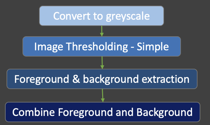
Obviously in method 1, we performed a lot of image processing. As can be seen, Gaussian Blur, and Otsu thresholding require a lot of processing. Additionally, when applying Gaussian Blur and binning, we lost a lot of detail in our image. Hence, we wanted to design an alternative strategy that will hopefully be faster. Balanced against efficiency and knowing OpenCV is a highly optimized library, we opted for a thresholding focused approach:

1. Convert our image into Greyscale
2. Perform simple thresholding to build a mask for the foreground and background
3. Determine the foreground and background based on the mask
4. Reconstruct original image by combining foreground and background

Given these points, our second background remover code ended up as follows:

def bgremove2(myimage):
    # First Convert to Grayscale
    myimage_grey = cv2.cvtColor(myimage, cv2.COLOR_BGR2GRAY)

    ret,baseline = cv2.threshold(myimage_grey,127,255,cv2.THRESH_TRUNC)

    ret,background = cv2.threshold(baseline,126,255,cv2.THRESH_BINARY)

    ret,foreground = cv2.threshold(baseline,126,255,cv2.THRESH_BINARY_INV)

    foreground = cv2.bitwise_and(myimage,myimage, mask=foreground)  # Update foreground with bitwise_and to extract real foreground

    # Convert black and white back into 3 channel greyscale
    background = cv2.cvtColor(background, cv2.COLOR_GRAY2BGR)

    # Combine the background and foreground to obtain our final image
    finalimage = background+foreground
    return finalimage

Background Remover with OpenCV – Method 3 – Working in HSV Color Space

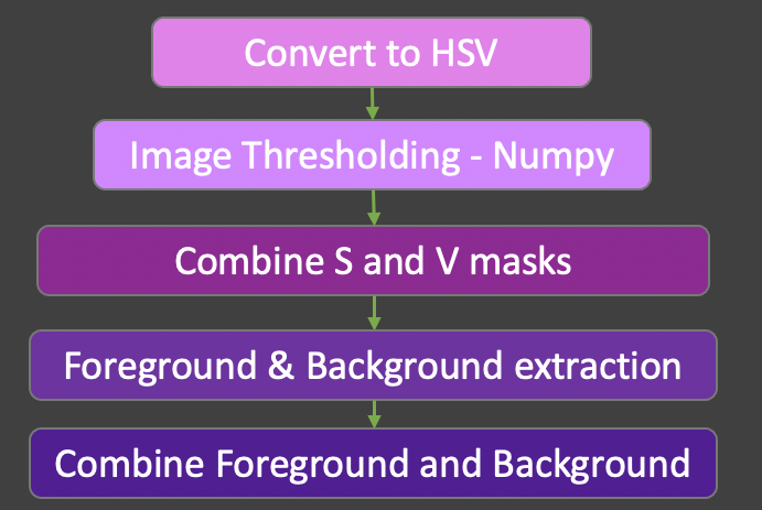
Until now, we have been working in BGR color space. With this in mind, our images are prone to poor lighting and shadows. Unquestionably, we wanted to know if working in HSV color space would render better results. In order not to lose image detail we also decided not to perform Gaussian Blur nor image binning. Instead to focus on Numpy for thresholding and generating image masks. Generally, our strategy was as follows:

1. Convert our image into HSV color space
2. Perform simple thresholding to create a map using Numpy based on Saturation and Value
3. Combine the map from S and V into a final mask
4. Determine the foreground and background based on the combined mask
5. Reconstruct original image by combining extracted foreground and background

Given these points, our third background remover code ended up as follows:

def bgremove3(myimage):
    # BG Remover 3
    myimage_hsv = cv2.cvtColor(myimage, cv2.COLOR_BGR2HSV)
    
    #Take S and remove any value that is less than half
    s = myimage_hsv[:,:,1]
    s = np.where(s < 127, 0, 1) # Any value below 127 will be excluded

    # We increase the brightness of the image and then mod by 255
    v = (myimage_hsv[:,:,2] + 127) % 255
    v = np.where(v > 127, 1, 0)  # Any value above 127 will be part of our mask

    # Combine our two masks based on S and V into a single "Foreground"
    foreground = np.where(s+v > 0, 1, 0).astype(np.uint8)  #Casting back into 8bit integer

    background = np.where(foreground==0,255,0).astype(np.uint8) # Invert foreground to get background in uint8
    background = cv2.cvtColor(background, cv2.COLOR_GRAY2BGR)  # Convert background back into BGR space
    foreground=cv2.bitwise_and(myimage,myimage,mask=foreground) # Apply our foreground map to original image
    finalimage = background+foreground # Combine foreground and background

    return finalimage

Results – Image Quality

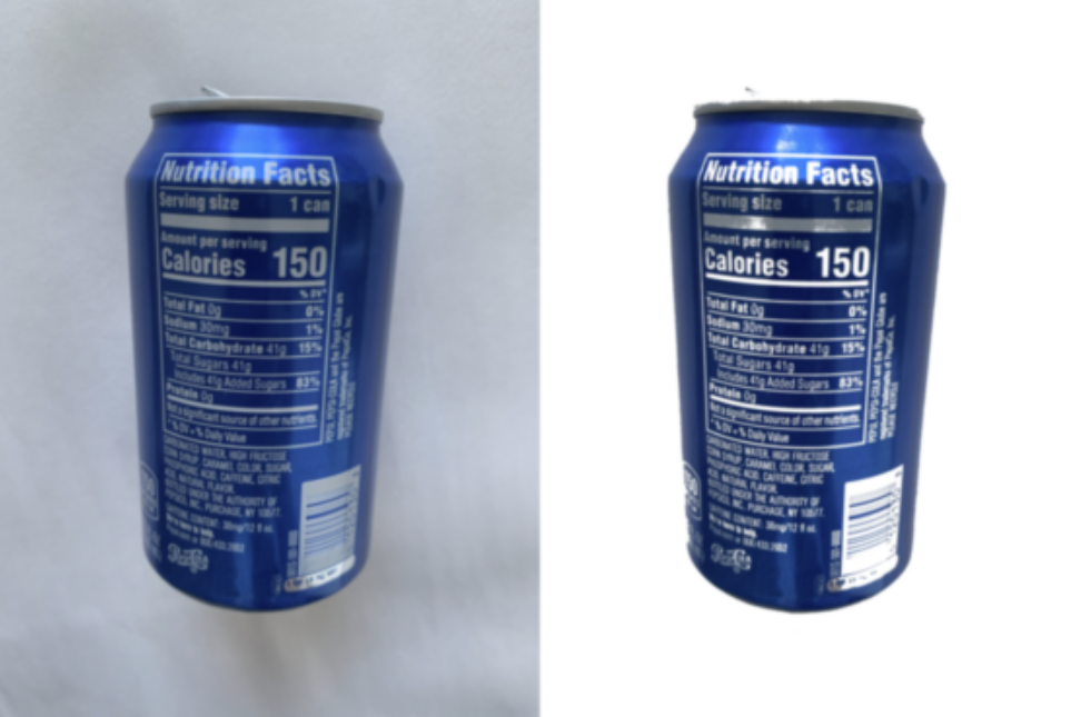
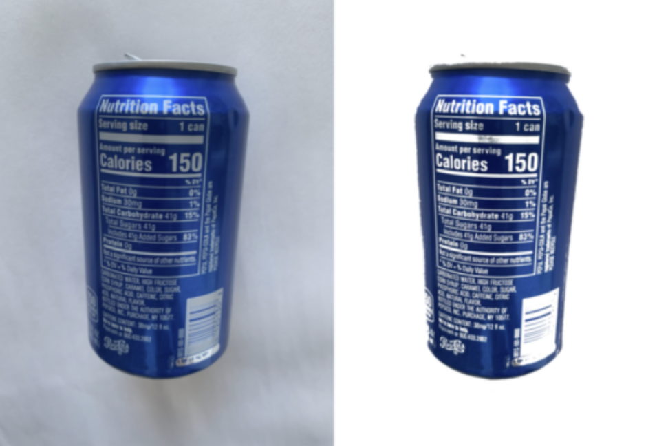
Up to the present time, we have shared three different background removers. Undoubtedly, you are wondering how they performed? Which one is better? In order to answer this question, we take a relatively simple image and compare the results.

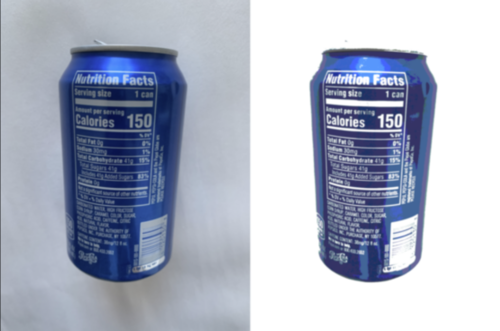
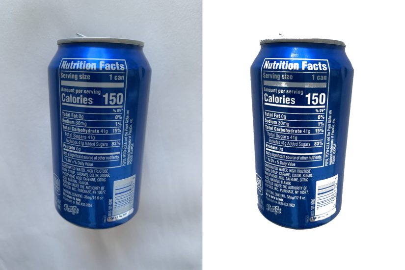
While it may be true, all three background removers were able to adequately remove the simple background in our original image. Unfortunately background remover 1 reduced the fidelity of our image. Furthermore the limited color range available reduced details such as the shine on the can. This is most apparent when examining the top and sides of the can. At the same time the top rim of the can was partially removed.

Whereas we perform blur and binning for background remover 1, we did not do so for remover 2. In this case we managed to preserve the finer details of the can surface and text are more clear. Surprisingly we improved the results by better preserving the top rim as well. Moreover, the contour of the can was sharper and better preserved.

Finally we examine the results of background remover 3. Generally the overall performance were good, again the surface details and text are crisp. By and large background remover 3 preserved the top rim of the can well. Compared to background remover 2 though, we lost some details in the barcode as well as having more fuzzy edges to the sides.

Results – System Performance

At this point, we wanted to compare system performance when using all three background removers. Even though the result of one may be better, dependent on our use case, performance may be more important. For this purpose, we timed the run time of the three background removers.

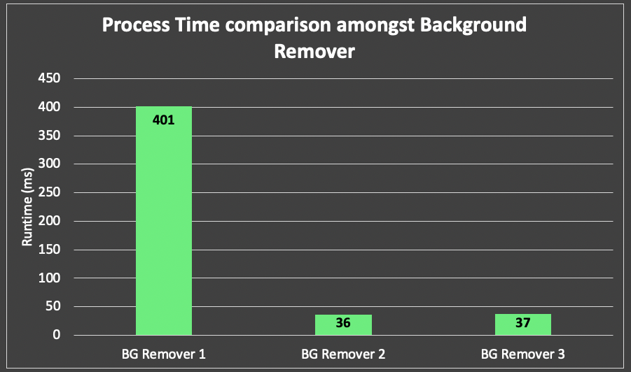
Since background remover 1 performed many computationally expensive operations, it was not surprising it take the most time. Especially with both gaussian blur and color binning operations. Consequently taking these out allowed us to reduce run time by 90% for both background mover 2 & 3. Comparatively, background remover 3 takes 1 ms longer to run. This can be explained by the fact more time was needed for two numpy operations (both S and V channels.)

Conclusions

If you followed us through our article to this point (or you jumped directly to the conclusion), then you will agree Background Remover 2 is the overall better approach. For the most part, it produced the best image clarity and preserved a lot of the material details. Nevertheless, it is important to realise that we used the mid point (of 8 bit – 256 value) for simple thresholding. Since this depends on simple thresholding on a greyscale image, we obtain the best results when using a white background. In other words, controlling how the image is taken solves half the problem.

Performing gaussian blur and color binning reduces image fidelity at high processing cost. This approach will only be beneficial in niche applications. Typically if image size or memory size is of priority, we can apply background remover 1 as a pre-processing step.

Another point to consider is how do we manage portions of the image similar to the background color. If we examine closely, then we will find background remover 3 did the best in preserving the shine on the top of the can. Evidently working in HSV space yielded better results when managing colors with high contrast. Consequently, we could improve our strategy by taking images with a high contrasting background. Instead of white, colors not part of the main object may be better. Subsequently, applying the “Four Corner” technique may provide better threshold values.

Last but not least, we can improve the performance further by leveraging GPUs. Current performance measures are CPU based. If we compiled our OpenCV libraries with CUDA, or leveraged Numba/JAX, then we can expect better results.

About Alan Wong Alan is a part time Digital enthusiast and full time innovator who believes in freedom for all via Digital Transformation.  兼職人工智能愛好者，全職企業家利用數碼科技釋放潛能與自由。